
[<link http: www.nature.com articles srep13495>Scientific Reports 5, 13495 (2015)]
The aim for understanding transport phenomena is at the heart of many studies on processes in nature and man-made structures ranging from photosynthesis to information network applications. Recent research indicates that the combination of classical with quantum effects can explain or introduce highly unexpected behaviour of the overall system. In order to understand quantum transport processes on a random or non-static network, as it can be found in molecules or porous media, quantum walks on a dynamical percolation graph can serve as an ideal test bed for exploring the boundaries between the classical and quantum regime. In a German-Czech collaboration scientist from the IQO group in Paderborn together with their theory partners from Prague have now found revivals of coherences of such a quantum walk, where they extended their <link>time-multiplexed quantum walk experiments by a dynamic coin operator realised with an electro-optic modulator.
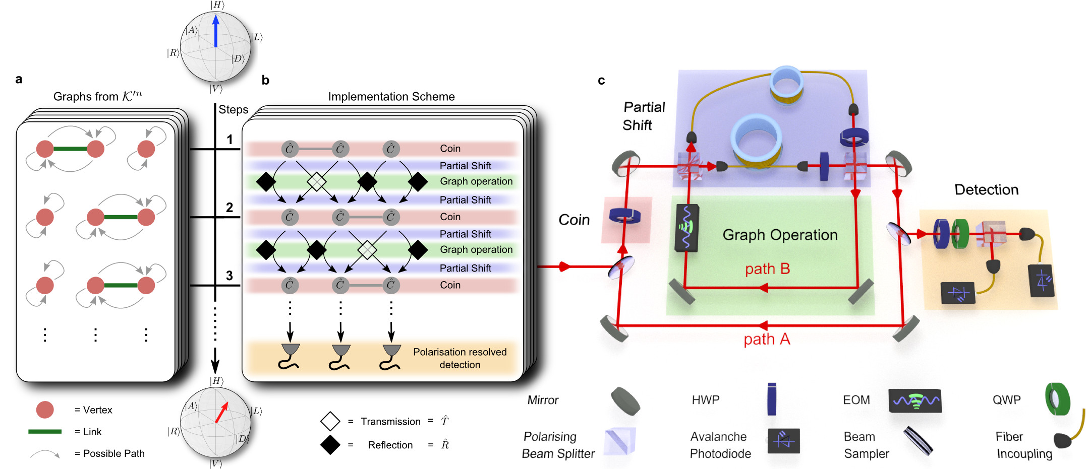
A quantum walk is a genuine quantum process taking place on a prescribed graph or network, consisting of vertices and links connecting them, and serves as an established model system for various quantum transport phenomena like photosynthesis. Up to now there exist many experimental implementations of quantum walks on static and fully connected graphs. However, percolation, a concept concerning the connectivity of random graphs, relies on the modification of the graph structure. The model has been extensively studied in mathematics and physics, with applications ranging from phase transitions to a multitude of transport phenomena. In the standard percolation model links between vertices of a finite graph are present or absent with a given probability, optimized to the simulation of randomly evolving --fluctuating media, networks or environments.
By exploiting a clever split-step scheme they managed to dynamically break links in the underlying graph. That means that the walker sees in every step of its dynamics another graph configuration with present or absent links, i.e. allowed or forbidden transmission, between the vertices of the graph.
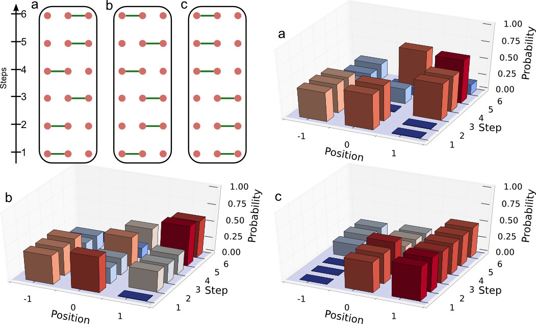
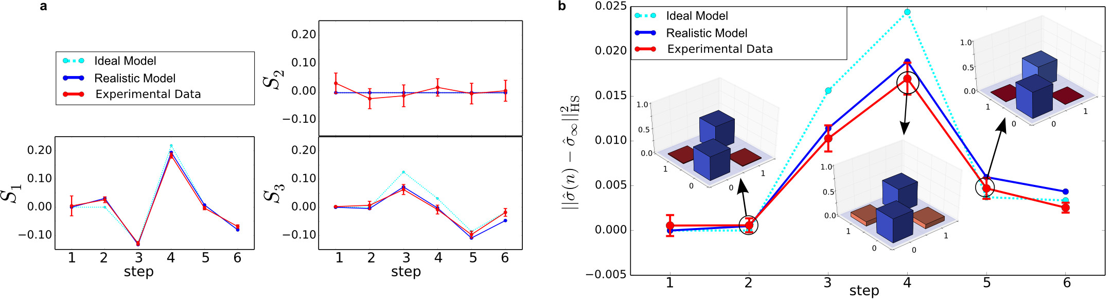
To test the capabilities of their setup they measured the coherences properties of a finite system consisting of 3 positions and link probability of 50%. For this they measured 64 different graph configurations and averaged over them. They tracked the evolution of the internal state of the walker tomographically and found that, although after one step the coherence seems to be destroyed and the walker is in the totally mixed state, there is a revival after 3 steps. Here the distance of the walker's state to the totally mixed state increases again, the coherence enlarges, a clear signature of non-Markovian dynamics. From theory exactly such a periodic dynamic is predicted, but contradicts the intuition that randomness will destroy the quantum interferences and cause a quantum-to-classical transition of the evolution. Such a transition to an incoherent process was found e.g. for random perturbations of the internal state of the walker (see <link>here).
The scientists have shown that even those subtle decoherence mechanisms in complex systems can be investigated within the quantum walk framework which proves the precise coin control and the stability of the time-multiplexing scheme.


